Exponential curve fitting in R
Solution 1
You need a model to fit to the data. Without knowing the full details of your model, let's say that this is an exponential growth model, which one could write as: y = a * e r*t
Where y is your measured variable, t is the time at which it was measured, a is the value of y when t = 0 and r is the growth constant. We want to estimate a and r.
This is a non-linear problem because we want to estimate the exponent, r. However, in this case we can use some algebra and transform it into a linear equation by taking the log on both sides and solving (remember logarithmic rules), resulting in: log(y) = log(a) + r * t
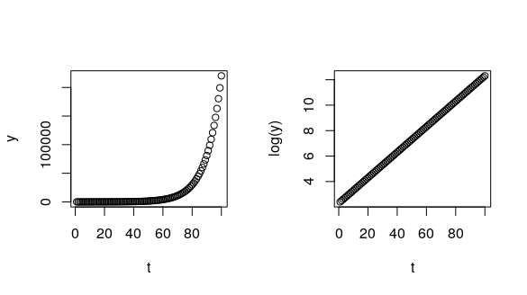
We can visualise this with an example, by generating a curve from our model, assuming some values for a and r:
t <- 1:100      # these are your time points
a <- 10         # assume the size at t = 0 is 10
r <- 0.1        # assume a growth constant
y <- a*exp(r*t) # generate some y observations from our exponential model
# visualise
par(mfrow = c(1, 2))
plot(t, y)      # on the original scale
plot(t, log(y)) # taking the log(y)
So, for this case, we could explore two possibilies:
- Fit our non-linear model to the original data (for example using
nls()function) - Fit our "linearised" model to the log-transformed data (for example using the
lm()function)
Which option to choose (and there's more options), depends on what we think (or assume) is the data-generating process behind our data.
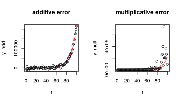
Let's illustrate with some simulations that include added noise (sampled from a normal distribution), to mimic real data. Please look at this StackExchange post for the reasoning behind this simulation (pointed out by Alejo Bernardin's comment).
set.seed(12) # for reproducible results
# errors constant across time - additive
y_add <- a*exp(r*t) + rnorm(length(t), sd = 5000) # or: rnorm(length(t), mean = a*exp(r*t), sd = 5000)
# errors grow as y grows - multiplicative (constant on the log-scale)
y_mult <- a*exp(r*t + rnorm(length(t), sd = 1))  # or: rlnorm(length(t), mean = log(a) + r*t, sd = 1)
# visualise
par(mfrow = c(1, 2))
plot(t, y_add, main = "additive error")
lines(t, a*exp(t*r), col = "red")
plot(t, y_mult, main = "multiplicative error")
lines(t, a*exp(t*r), col = "red")
For the additive model, we could use nls(), because the error is constant across
t. When using nls() we need to specify some starting values for the optimization algorithm (try to "guesstimate" what these are, because nls() often struggles to converge on a solution).
add_nls <- nls(y_add ~ a*exp(r*t),
               start = list(a = 0.5, r = 0.2))
coef(add_nls)
#           a           r
# 11.30876845  0.09867135
Using the coef() function we can get the estimates for the two parameters.
This gives us OK estimates, close to what we simulated (a = 10 and r = 0.1).
You could see that the error variance is reasonably constant across the range of the data, by plotting the residuals of the model:
plot(t, resid(add_nls))
abline(h = 0, lty = 2)
For the multiplicative error case (our y_mult simulated values), we should use lm() on log-transformed data, because
the error is constant on that scale instead.
mult_lm <- lm(log(y_mult) ~ t)
coef(mult_lm)
# (Intercept)           t
#  2.39448488  0.09837215
To interpret this output, remember again that our linearised model is log(y) = log(a) + r*t, which is equivalent to a linear model of the form Y = β0 + β1 * X, where β0 is our intercept and β1 our slope.
Therefore, in this output (Intercept) is equivalent to log(a) of our model and t is the coefficient for the time variable, so equivalent to our r.
To meaningfully interpret the (Intercept) we can take its exponential (exp(2.39448488)), giving us ~10.96, which is quite close to our simulated value.
It's worth noting what would happen if we'd fit data where the error is multiplicative
using the nls function instead:
mult_nls <- nls(y_mult ~ a*exp(r*t), start = list(a = 0.5, r = 0.2))
coef(mult_nls)
#            a            r
# 281.06913343   0.06955642
Now we over-estimate a and under-estimate r (Mario Reutter highlighted this in his comment). We can visualise the consequence of using the wrong approach to fit our model:
# get the model's coefficients
lm_coef <- coef(mult_lm)
nls_coef <- coef(mult_nls)
# make the plot
plot(t, y_mult)
lines(t, a*exp(r*t), col = "brown", lwd = 5)
lines(t, exp(lm_coef[1])*exp(lm_coef[2]*t), col = "dodgerblue", lwd = 2)
lines(t, nls_coef[1]*exp(nls_coef[2]*t), col = "orange2", lwd = 2)
legend("topleft", col = c("brown", "dodgerblue", "orange2"),
       legend = c("known model", "nls fit", "lm fit"), lwd = 3)
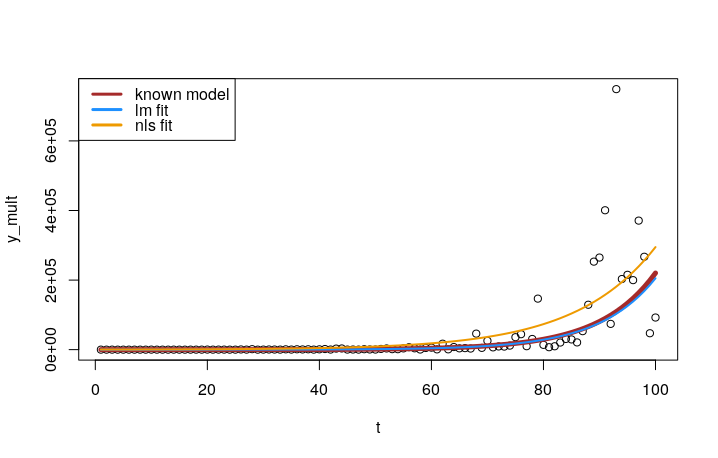
We can see how the lm() fit to log-transformed data was substantially better than the nls() fit on the original data.
You can again plot the residuals of this model, to see that the variance is not constant across the range of the data (we can also see this in the graphs above, where the spread of the data increases for higher values of t):
plot(t, resid(mult_nls))
abline(h = 0, lty = 2)
Solution 2
Unfortunately taking the logarithm and fitting a linear model is not optimal. The reason is that the errors for large y-values weight much more than those for small y-values when apply the exponential function to go back to the original model. Here is one example:
f <- function(x){exp(0.3*x+5)}
squaredError <- function(a,b,x,y) {sum((exp(a*x+b)-f(x))^2)}
x <- 0:12
y <- f(x) * ( 1 + sample(-300:300,length(x),replace=TRUE)/10000 )
x
y
#--------------------------------------------------------------------
M <- lm(log(y)~x)
a <- unlist(M[1])[2]
b <- unlist(M[1])[1]
print(c(a,b))
squaredError(a,b,x,y)
approxPartAbl_a <- (squaredError(a+1e-8,b,x,y) - squaredError(a,b,x,y))/1e-8
for ( i in 0:10 )
{
  eps <- -i*sign(approxPartAbl_a)*1e-5
  print(c(eps,squaredError(a+eps,b,x,y)))
}
Result:
> f <- function(x){exp(0.3*x+5)}
> squaredError <- function(a,b,x,y) {sum((exp(a*x+b)-f(x))^2)}
> x <- 0:12
> y <- f(x) * ( 1 + sample(-300:300,length(x),replace=TRUE)/10000 )
> x
 [1]  0  1  2  3  4  5  6  7  8  9 10 11 12
> y
 [1]  151.2182  203.4020  278.3769  366.8992  503.5895  682.4353  880.1597 1186.5158 1630.9129 2238.1607 3035.8076 4094.6925 5559.3036
> #--------------------------------------------------------------------
>
> M <- lm(log(y)~x)
> a <- unlist(M[1])[2]
> b <- unlist(M[1])[1]
> print(c(a,b))
          coefficients.x coefficients.(Intercept)
               0.2995808                5.0135529
> squaredError(a,b,x,y)
[1] 5409.752
> approxPartAbl_a <- (squaredError(a+1e-8,b,x,y) - squaredError(a,b,x,y))/1e-8
> for ( i in 0:10 )
+ {
+   eps <- -i*sign(approxPartAbl_a)*1e-5
+   print(c(eps,squaredError(a+eps,b,x,y)))
+ }
[1]    0.000 5409.752
[1]   -0.00001 5282.91927
[1]   -0.00002 5157.68422
[1]   -0.00003 5034.04589
[1]   -0.00004 4912.00375
[1]   -0.00005 4791.55728
[1]   -0.00006 4672.70592
[1]   -0.00007 4555.44917
[1]   -0.00008 4439.78647
[1]   -0.00009 4325.71730
[1]   -0.0001 4213.2411
>
Perhaps one can try some numeric method, i.e. gradient search, to find the minimum of the squared error function.
Solution 3
If it really is exponential, you can try taking the logarithm of your variable and fitting a linear model to that.
Related videos on Youtube
 07 : 40
Si22
Updated on July 31, 2022Comments
-
 Si22 4 months
time = 1:100
head(y)
0.07841589 0.07686316 0.07534116 0.07384931 0.07238699 0.07095363
plot(time,y)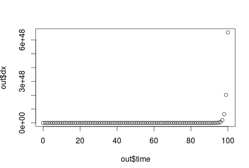
This is an exponential curve.
-
How can I fit line on this curve without knowing the formula ? I can't use 'nls' as the formula is unknown (only data points are given).
-
How can I get the equation for this curve and determine the constants in the equation?
I tried loess but it doesn't give the intercepts.
-
-
 Alejo Bernardin almost 5 yearsIf someone wants to know more about when to use
lm()ornls(), here there is a good discussion stats.stackexchange.com/questions/61747/… -
 Mario Reutter almost 3 yearsFitting a linear model to logarithmized values (with
lm) yields a different result than fitting the non-linear model (withnls) because different distances are minimized. For the logarithmized linear model, the logarithmized residuals are minimized, creating a bias away from bigger remaining residuals. Hence, the onset of the growth will more easily be mis-estimated. -
hugot over 2 years@wpkzz yes the original answer was fundamentally wrong. I've completely re-written it now, hoping it's accurate. Thanks for highlighting this problem (coming back to it 5 years later is rather humbling...)
-
 Rodrigo over 2 yearsA graph would have greatly enhanced your answer.