How to get VLOOKUP to return the *last* match?
Solution 1
You can use an array formula to get data from the last matching record.
=INDEX(IF($A$1:$A$20="c",$B$1:$B$20),MAX(IF($A$1:$A$20="c",ROW($A$1:$A$20))))
Enter the formula using Ctrl+Shift+Enter.
This works like the INDEX/MATCH construction of a VLOOKUP, but with a conditional MAX used instead of MATCH.
Note that this assumes that your table starts at row 1. If your data starts at a different row, you will need to adjust the ROW(...) part by subtracting the difference between the top row and 1.
Solution 2
(Answering here as no separate question for sorted data.)
If the data were sorted, you could use VLOOKUP with the range_lookup argument TRUE (or omitted, since it's the default), which is officially described for Excel as "search for approximate match".
In other words, for sorted data:
- setting the last argument to
FALSEreturns the first value, and - setting the last argument to
TRUEreturns the last value.
This is largely undocumented and obscure, but dates to VisiCalc (1979), and today holds at least in Microsoft Excel, LibreOffice Calc, and Google Sheets. It is ultimately due to the initial implementation of LOOKUP in VisiCalc (and thence VLOOKUP and HLOOKUP), when there was no fourth parameter. The value is found by binary search, using inclusive left bound and exclusive right bound (a common and elegant implementation), which results in this behavior.
Technically this means that one starts the search with the candidate interval [0, n), where n is the length of the array, and the loop invariant condition is that A[imin] <= key && key < A[imax] (the left bound is <= the target, the right bound, which starts one after the end, is > the target; to validate, either check values at endpoints before, or check result after), and successively bisecting and choosing whichever side preserves this invariant: by exclusion one side will, until you get to an interval with 1 term, [k, k+1), and the algorithm then returns k. This need not be an exact match (!): it's just the closest match from below. In case of duplicate matches, this results in returning the last match, as it requires that the next value be greater than the key (or the end of the array). In case of duplicates you need some behavior, and this is reasonable and easy to implement.
This behavior is stated explicitly in this old Microsoft Knowledge Base article (emphasis added): "XL: How to Return the First or Last Match in an Array" (Q214069):
You can use the LOOKUP() function to search for a value within an array of sorted data and return the corresponding value contained in that position within another array. If the lookup value is repeated within the array, it returns the last match encountered. This behavior is true for the VLOOKUP(), HLOOKUP(), and LOOKUP() functions.
Official documentation for some spreadsheets follow; in neither is the "last match" behavior stated, but it's implied in the Google Sheets documentation:
-
TRUE assumes the first column in the table is sorted either numerically or alphabetically, and will then search for the closest value.
-
If
is_sortedisTRUEor omitted, the nearest match (less than or equal to the search key) is returned
Solution 3
If the values in the search array are sequential (i.e. you're looking for the largest value, such as the latest date), you don't even need to use the INDIRECT function. Try this simple code:
=MAX(IF($A$1:$A$20="c",$B$1:$B$20,)
Again, enter the formula using CTRL + SHIFT + ENTER
Related videos on Youtube
 08 : 54
 06 : 19
 21 : 15
 07 : 38
 14 : 13
Murray Furtado
Hello, world! I enjoy using my experience to help others. That is why I am active at a number of other sites in the StackExchange network on topics that interest me. I'm something of a Swiss army knife both professionally and in private, able to juggle a wild variety of things at once. I've worked in every kind of business that uses software. I'm also very good with tools, both IT and mechanic. Whether you need software design or assembling some IKEA furniture, I'm your man for the job. I'm generally soft-spoken but driven by clear principles. I'm a twin, I've lived in five countries, I speak four languages fluently and two more embarrassingly. Also, being a father routinely develops my patience which is useful for moderating on StackExchange too. To learn more about me, see my Google+ profile.
Updated on September 18, 2022Comments
-
Murray Furtado over 1 year
I'm used to working with VLOOKUP but this time I have a challenge. I don't want the first matching value, but the last. How? (I'm working with LibreOffice Calc but an MS Excel solution ought to be equally useful.)
The reason is that I have two text columns with thousands of rows, let's say one is a list of transaction payees (Amazon, Ebay, employer, grocery store, etc.) and the other is a list of spending categories (wages, taxes, household, rent, etc.). Some transactions don't have the same spending category every time, and I want to grab the most recently used one. Note that the list is sorted by neither column (in fact by date), and I don't want to change the sort order.
What I have (excluding error handling) is the usual "first-match" formula:
=VLOOKUP(
[payee field] , [payee+category range] , [index of category column] ,
0 )
I've seen solutions like this, but I get
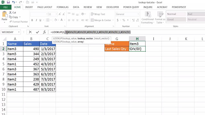
#DIV/0!errors:=LOOKUP(2 , 1/( [payee range] = [search value] ) , [category range] )The solution can be any formula, not necessarily VLOOKUP. I can also swap the payee/category columns around. Just no change in sorting column, please.
Bonus points for a solution that picks the most frequent value rather than the last!
-
Murray Furtado almost 10 yearsI'm confused about that literal "c" - I'd think that the evaluation is always false, so what does it really do?
-
Murray Furtado almost 10 yearsI've tested your suggestion (and checked that it was accepted as an array formula). I assume Col A is payee and B is category, right? Unfortunately, LibreOffice returns "ERR:502" which translates into "Invalid argument: Function argument is not valid. For example, a negative number for the SQRT() function, for this please use IMSQRT()". I checked that all the functions exist with that name in LibreOffice, but I wonder whether LibreOffice's
IFcan't handle arrays. -
 Excellll almost 10 yearsSorry, the literal "c" was just the payee name you wanted to match. That was a relic from my sample data I was playing with. I assume that will be replaced with a cell reference in your sheet.
 -
Excellll almost 10 years@TorbenGundtofte-Bruun Care to share the formula you're using? I may be able to troubleshoot it if I can see it. Also, you can always try to step through the formula with
Evaluate Formulato see which part of the formula is generating the error. This feature exists in Excel, and I'd be surprised if LibreOffice Calc doesn't have the same feature. -
Murray Furtado almost 10 yearsMy original formula is straightforward, that's why it's not adequate :-)
=VLOOKUP(J1061;$J$2:$K$9999;2;0)where col J contains payees and col K the categories. It returns the first match as expected. -
Murray Furtado almost 10 yearsMy formula based on your suggestion is:
=INDEX(IF($J$2:$J$9999=J1061;$K$2:$K$9999);MAX(IF($J$2:$J$9999=J1061;ROW($J$2:$J$9999)))) -
Excellll almost 10 years@TorbenGundtofte-Bruun Your data starts at row 2, so you need to adjust the
ROW()part of the formula by subtracting 1 to make the indices and row numbers match. New formula to try:=INDEX(IF($J$2:$J$9999=J1061;$K$2:$K$9999);MAX(IF($J$2:$J$9999=J1061;ROW($J$2:$J$9999)-1))) -
Máté Juhász over 8 years
LOOKUPworks only on sorted list, the output of your comarison will result in a list of1s and spaces in a non-sorted way, so it won't give correct result. -
davetapley about 6 yearsThat nearest match thing was driving me crazy!