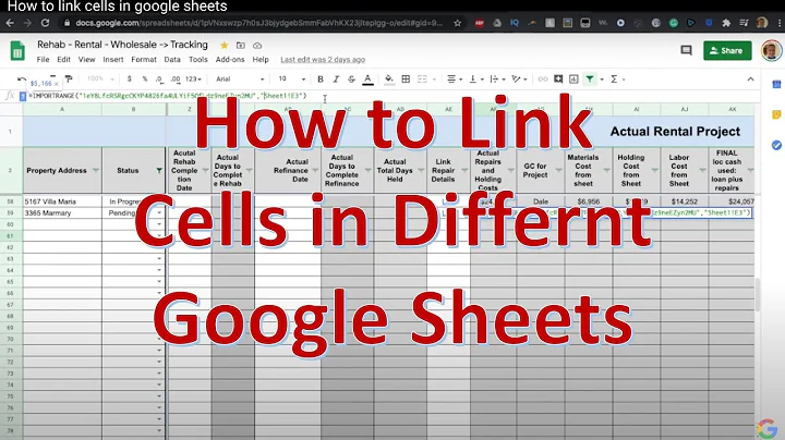
How to insert hyperlink to a cell in Google sheet using formula?

Question

I am trying to insert a hyperlink to a cell in a fashion that can be replicated using '=MATCH()" function. However, I can't seem to figure out a method to link a cell in Google sheets without using the GID.

When I right-click and "Get link to this cell" I get a URL with "#gid=1933185132" in the end. However this has no structure and I can't use it with a MATCH formula and autofill this like I normally do in Excel.

https://docs.google.com/spreadsheets/d/sheetkey/edit#gid=1933185132

However if this is has a cell reference like so

https://docs.google.com/spreadsheets/d/sheetkey/edit#Sheet1!C12

I can easily recreate it for the MATCH function.

Question: Is there an alternate way to link cell like I have shown above? If not Can I use a formula to extract the GID of "Sheet1!C12"?

I have searched the google forums and stack overflow to the best of my extent and the only solutions I saw seemed to use scripts with "var sheet" something which I cant make sense of having 0 knowledge of coding.

It should be a very straightforward thing to do, but I am not able to find a way out. Any insight into the issue is appreciated. Thank you very much.

Solution 1

Range

You can create a link like this:

=hyperlink("#gid=1166414895range=A1", "link to A1")

Each tab has a unique key, called gid, you'll find it in the link:

• #gid will never change. Tab name may be changed and the formula will break, using gid is safer.
• A1 is a part you need to find using match, address functions to get dynamic links.

I could not find a documentation on this topic, and could not find a method using tab names.

Named Range

1. Define a named range in the document.
2. In a cell select "Insert link".
3. In the link dialog box, select "Named ranges in this spreadsheet."
4. Select the name of the range created in step 1.
5. Click the "Apply" button.
6. Move mouse pointer over the new link. A pop-up containing a link like "#rangeid=nnnnnnnnnn" will appear.
7. Right click on the link in the pop-up to open your browser's contextual menu.
8. Select the "Copy Link Address" or just "Copy" function.

Depending on your browser, your clipboard will now contain either the full URL:

https://docs.google.com/spreadsheets/d/xxxxxxxxxx/edit#rangeid=nnnnnnnnnn

Or the clipboard will have just the range ID fragment:

#rangeid=nnnnnnnnnn

If you have only the fragment, you'll need to append it to the URL of the document to create a complete URL for the range.

There may be some other, simpler way to get the range ID, but I've not noticed one yet. See related question, answer to a similar question.

PS: After you've copied the URL for the named range, you may delete the link that was created by following the steps above.

Custom functions

Use in a formula.

Simple range:

=HYPERLINK(getLinkByRange("Sheet1","A1"), "Link to A1")

Named range:

=HYPERLINK(getLinkByNamedRange("NamedRange"), "Link to named range")

The code, insert into the script editor (Tools > Script Editor):

function getLinkByRange(sheetName, rangeA1, fileId)
{
  // file + sheet
  var file = getDafaultFile_(fileId);  
  var sheet = file.getSheetByName(sheetName);
  
  return getCombinedLink_(rangeA1, sheet.getSheetId(), fileId, file)    
}

function getLinkByNamedRange(name, fileId)
{
  // file + range + sheet
  var file = getDafaultFile_(fileId);    
  var range = file.getRangeByName(name);  
  var sheet = range.getSheet();
  
  return getCombinedLink_(range.getA1Notation(), sheet.getSheetId(), fileId, file)
      
}


function getDafaultFile_(fileId)
{
  // get file
  var file;
  if (fileId) { file = SpreadsheetApp.openById(fileId); }
  else file = SpreadsheetApp.getActive();      
  return file;      
}

function getCombinedLink_(rangeA1, sheetId, fileId, file)
{
  var externalPart = '';
  if (fileId) { externalPart = file.getUrl(); }    
  return externalPart + '#gid=' + sheetId + 'range=' + rangeA1;   
}

Solution 2

GID does not require to be a valid URL starting with https...

all you need is hyperlink it like:

=HYPERLINK("#gid=1933185132&range=C12", "sheet name")

---

and if you want to hyperlink all your sheets you can do it like this:

function SHEETLIST() {
try {
  var sheets = SpreadsheetApp.getActiveSpreadsheet().getSheets()
  var out = new Array( sheets.length+1 ) ;
  out[0] = [ "NAME" , "#GID" ];
  for (var i = 1 ; i < sheets.length+1 ; i++ ) out[i] = 
  [sheets[i-1].getName() , sheets[i-1].getSheetId() ];
  return out
}
catch( err ) {
  return "#ERROR!" 
}
}

---

=ARRAYFORMULA(HYPERLINK("#gid="&
 QUERY(INDEX(SHEETLIST();;2); "offset 1"); 
 QUERY(INDEX(SHEETLIST();;1); "offset 1")))

Solution 3

Since the URL upto the following part is going to be a constant, you can define it in a cell first.

https://docs.google.com/spreadsheets/d/sheetkey/edit#

I believe you already have the gid=1933185132 part defined in a column (let's say its column A). So to get the actual URL of the sheet, you just have to concatenate these two. So in the column B you have to write the following formula.

=HYPERLINK(CONCAT(A1,A2),A2)