LibreOffice Calc: conditional formatting based of column / cell value

Question

Unfortunately I cannot grasp how the conditional formatting works. I have a sheet like that:

I have defined 2 cell styles "Low" and "High" and I want cells in columns A-E to have one of these styles applied if the cell in column G has a value "L" or "H" respectively. If anything else is put there the cells shall stay white as they are.

For the demonstration purposes I a have manually applied the styles to the example rows.

Perhaps I am doing something wrong, but whatever I do either some cells do not have the proper style applied or some other cells have the style also applied. I was not able to achieve the desired result.

Could you please describe the exact steps to obtain the desired formatting...

Solution 1

I am using LibreOffice Calc 5.1.6.2.

Just like my highly respected preceding poster described:

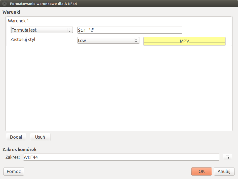
1. Select the range of cells to be conditionally formatted (in my case A1:F44);
2. Select Menu Format -> Conditional Formatting -> Manage...:
3. Add first colouring:

Formula is $G1="H"

Note: the dollar sign is important here! Denotes un-relative column reference to column G, as opposed to the relative row reference 1. Relative means that the reference changes as the Calc evaluator moves down the sheet rows.

4. Press OK and Add the second colouring:

5. Now your conditional formatting should look like this:

6. And voilà - now all out of norm rows get properly highlighted:

Please note that entering 2 conditions in one conditional format does not work properly - probably because of some residual formats trailing behind and changing some undesired fields. Actually right from the beginning I was lacking "else" condition.

Solution 2

For LibreOffice 5.1 as well as 6.0:

1. Select the range of cells to be conditionally formatted (e.g. A3:F50);
2. Select Menu Format -> Conditional Formatting -> Manage...:
3. Click Add:
4. Under "Condition 1", select "Formula is"; in the textbox, enter $G3="L"; next to "Apply style", select your style for "L" rows: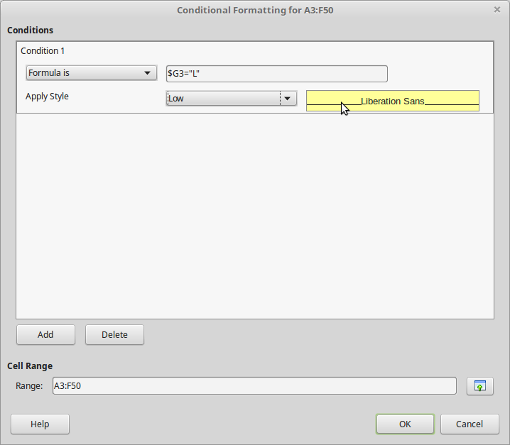
5. Click Add
6. Under "Condition 2", select "Formula is"; in the textbox, enter $G3="H"; next to "Apply style", select your style for "H" rows: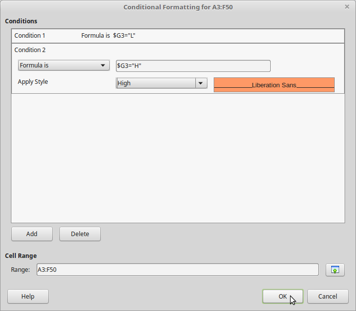
7. Click OK:
8. Click OK

Additional notes:

• take care to remove any other definitions for conditional formatting if there's still anything defined but not required;

• take care to select the range to be formatted first, and call Menu Format -> Conditional Formatting -> Manage... afterwards. the conditional formatting dialogue contains a field "Cell Range" that lures users to enter the cell range there - this won't work, i've already filed a bug report...

Comments

[Pawel Debski]

Thanks for you valuable post. Actually it does not work with Conditon 1 and Condition 2 - some othe cells get coloured as well (I do not know why). However based on your input I found the solution. I'll post it in a few minutes.