Summing data in rows based on horizontal and vertical criteria
10,361
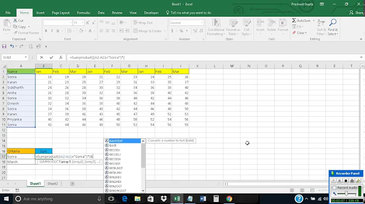
With the following setup:

I used the following formula
=SUMIF($B$1:$H$1,B$10,INDIRECT("$B" & MATCH($A11,$A$1:$A$5,0) & ":$H" &MATCH($A11,$A$1:$A$5,0)))
To get what was wanted. I put the formula in B11 and then copied across and Down
Related videos on Youtube
 10 : 54
Excel SUMIFS: Sum Alternate Columns based on Criteria and Header
 08 : 45
How To Sum Data With Multiple Vertical and Horizontal Criteria Using SUMPRODUCT Or SUMIFS In Excel
 10 : 55
Excel SUMPRODUCT with Criteria: SUM Alternate Columns based on Header and Criteria
 02 : 53
Sumif's On Rows and Columns for Excel And Google Sheets
 03 : 23
Sum based on row & column criteria in Excel
 14 : 04
Excel SUMIFS (better version of SUMIF), COUNTIFS & AVERAGEIFS (Multiple Criteria)
Author by
Lottie
Updated on June 14, 2022Comments
-
Lottie almost 2 years
I have a dataset in the below format:
           Date 1   Date 1   Date 1  Date 2   Date 2   Date 3   Date 3
Product 1    10       20       10      5       10       20       30
Product 2    5        5        10      10      10       5        30
Product 3    30       10       5       10      30       30       40
Product 4    5        10       10      20      5        10       20
and I am trying to sum the sales of the products by the date, to create the below:
           Date 1   Date 2   Date 3
Product 1    40       15       50
Product 3    45       40       70
Product 4    25       25       30
Product 2    20       20       35
The products in the second table will often be in a different order, so a simple
SUMIFwill not suffice.I've attempted a combination of
SUM,INDEXandMATCH, as well asSUMwith nestedIFfunction, but no amount of Googling or trial and error is getting me there. I keep just bringing back the values in one cell, but not managing to sum.-
Lottie over 8 yearsI didn't realise I was jumping into such a minefield. I thought I'd sign up as on top of 'general Excel' I also use VBA, HTML, CSS & JS so thought SO might be a bit of a one stop shop for any questions I might have!
-
 Richard Erickson over 8 years@pnuts Thanks for pointing that out. Do you if it would be possible to include that guidance on the Excel tag?
-