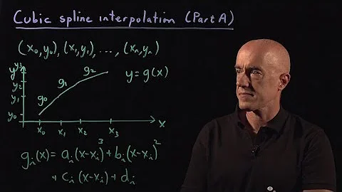
How to perform cubic spline interpolation in python?

Question

I have two lists to describe the function y(x):

x = [0,1,2,3,4,5]
y = [12,14,22,39,58,77]

I would like to perform cubic spline interpolation so that given some value u in the domain of x, e.g.

u = 1.25

I can find y(u).

I found this in SciPy but I am not sure how to use it.

Solution 1

Short answer:

from scipy import interpolate

def f(x):
    x_points = [ 0, 1, 2, 3, 4, 5]
    y_points = [12,14,22,39,58,77]

    tck = interpolate.splrep(x_points, y_points)
    return interpolate.splev(x, tck)

print(f(1.25))

Long answer:

scipy separates the steps involved in spline interpolation into two operations, most likely for computational efficiency.

1. The coefficients describing the spline curve are computed, using splrep(). splrep returns an array of tuples containing the coefficients.

2. These coefficients are passed into splev() to actually evaluate the spline at the desired point x (in this example 1.25). x can also be an array. Calling f([1.0, 1.25, 1.5]) returns the interpolated points at 1, 1.25, and 1,5, respectively.

This approach is admittedly inconvenient for single evaluations, but since the most common use case is to start with a handful of function evaluation points, then to repeatedly use the spline to find interpolated values, it is usually quite useful in practice.

Solution 2

In case, scipy is not installed:

import numpy as np
from math import sqrt

def cubic_interp1d(x0, x, y):
    """
    Interpolate a 1-D function using cubic splines.
      x0 : a float or an 1d-array
      x : (N,) array_like
          A 1-D array of real/complex values.
      y : (N,) array_like
          A 1-D array of real values. The length of y along the
          interpolation axis must be equal to the length of x.

    Implement a trick to generate at first step the cholesky matrice L of
    the tridiagonal matrice A (thus L is a bidiagonal matrice that
    can be solved in two distinct loops).

    additional ref: www.math.uh.edu/~jingqiu/math4364/spline.pdf 
    """
    x = np.asfarray(x)
    y = np.asfarray(y)

    # remove non finite values
    # indexes = np.isfinite(x)
    # x = x[indexes]
    # y = y[indexes]

    # check if sorted
    if np.any(np.diff(x) < 0):
        indexes = np.argsort(x)
        x = x[indexes]
        y = y[indexes]

    size = len(x)

    xdiff = np.diff(x)
    ydiff = np.diff(y)

    # allocate buffer matrices
    Li = np.empty(size)
    Li_1 = np.empty(size-1)
    z = np.empty(size)

    # fill diagonals Li and Li-1 and solve [L][y] = [B]
    Li[0] = sqrt(2*xdiff[0])
    Li_1[0] = 0.0
    B0 = 0.0 # natural boundary
    z[0] = B0 / Li[0]

    for i in range(1, size-1, 1):
        Li_1[i] = xdiff[i-1] / Li[i-1]
        Li[i] = sqrt(2*(xdiff[i-1]+xdiff[i]) - Li_1[i-1] * Li_1[i-1])
        Bi = 6*(ydiff[i]/xdiff[i] - ydiff[i-1]/xdiff[i-1])
        z[i] = (Bi - Li_1[i-1]*z[i-1])/Li[i]

    i = size - 1
    Li_1[i-1] = xdiff[-1] / Li[i-1]
    Li[i] = sqrt(2*xdiff[-1] - Li_1[i-1] * Li_1[i-1])
    Bi = 0.0 # natural boundary
    z[i] = (Bi - Li_1[i-1]*z[i-1])/Li[i]

    # solve [L.T][x] = [y]
    i = size-1
    z[i] = z[i] / Li[i]
    for i in range(size-2, -1, -1):
        z[i] = (z[i] - Li_1[i-1]*z[i+1])/Li[i]

    # find index
    index = x.searchsorted(x0)
    np.clip(index, 1, size-1, index)

    xi1, xi0 = x[index], x[index-1]
    yi1, yi0 = y[index], y[index-1]
    zi1, zi0 = z[index], z[index-1]
    hi1 = xi1 - xi0

    # calculate cubic
    f0 = zi0/(6*hi1)*(xi1-x0)**3 + \
         zi1/(6*hi1)*(x0-xi0)**3 + \
         (yi1/hi1 - zi1*hi1/6)*(x0-xi0) + \
         (yi0/hi1 - zi0*hi1/6)*(xi1-x0)
    return f0

if __name__ == '__main__':
    import matplotlib.pyplot as plt
    x = np.linspace(0, 10, 11)
    y = np.sin(x)
    plt.scatter(x, y)

    x_new = np.linspace(0, 10, 201)
    plt.plot(x_new, cubic_interp1d(x_new, x, y))

    plt.show()

Solution 3

If you have scipy version >= 0.18.0 installed you can use CubicSpline function from scipy.interpolate for cubic spline interpolation.

You can check scipy version by running following commands in python:

#!/usr/bin/env python3
import scipy
scipy.version.version

If your scipy version is >= 0.18.0 you can run following example code for cubic spline interpolation:

#!/usr/bin/env python3

import numpy as np
from scipy.interpolate import CubicSpline

# calculate 5 natural cubic spline polynomials for 6 points
# (x,y) = (0,12) (1,14) (2,22) (3,39) (4,58) (5,77)
x = np.array([0, 1, 2, 3, 4, 5])
y = np.array([12,14,22,39,58,77])

# calculate natural cubic spline polynomials
cs = CubicSpline(x,y,bc_type='natural')

# show values of interpolation function at x=1.25
print('S(1.25) = ', cs(1.25))

## Aditional - find polynomial coefficients for different x regions

# if you want to print polynomial coefficients in form
# S0(0<=x<=1) = a0 + b0(x-x0) + c0(x-x0)^2 + d0(x-x0)^3
# S1(1< x<=2) = a1 + b1(x-x1) + c1(x-x1)^2 + d1(x-x1)^3
# ...
# S4(4< x<=5) = a4 + b4(x-x4) + c5(x-x4)^2 + d5(x-x4)^3
# x0 = 0; x1 = 1; x4 = 4; (start of x region interval)

# show values of a0, b0, c0, d0, a1, b1, c1, d1 ...
cs.c

# Polynomial coefficients for 0 <= x <= 1
a0 = cs.c.item(3,0)
b0 = cs.c.item(2,0)
c0 = cs.c.item(1,0)
d0 = cs.c.item(0,0)

# Polynomial coefficients for 1 < x <= 2
a1 = cs.c.item(3,1)
b1 = cs.c.item(2,1)
c1 = cs.c.item(1,1)
d1 = cs.c.item(0,1)

# ...

# Polynomial coefficients for 4 < x <= 5
a4 = cs.c.item(3,4)
b4 = cs.c.item(2,4)
c4 = cs.c.item(1,4)
d4 = cs.c.item(0,4)

# Print polynomial equations for different x regions
print('S0(0<=x<=1) = ', a0, ' + ', b0, '(x-0) + ', c0, '(x-0)^2  + ', d0, '(x-0)^3')
print('S1(1< x<=2) = ', a1, ' + ', b1, '(x-1) + ', c1, '(x-1)^2  + ', d1, '(x-1)^3')
print('...')
print('S5(4< x<=5) = ', a4, ' + ', b4, '(x-4) + ', c4, '(x-4)^2  + ', d4, '(x-4)^3')

# So we can calculate S(1.25) by using equation S1(1< x<=2)
print('S(1.25) = ', a1 + b1*0.25 + c1*(0.25**2) + d1*(0.25**3))

# Cubic spline interpolation calculus example
    #  https://www.youtube.com/watch?v=gT7F3TWihvk

Solution 4

Just putting this here if you want a dependency-free solution.

Code taken from an answer above: https://stackoverflow.com/a/48085583/36061

def my_cubic_interp1d(x0, x, y):
    """
    Interpolate a 1-D function using cubic splines.
      x0 : a 1d-array of floats to interpolate at
      x : a 1-D array of floats sorted in increasing order
      y : A 1-D array of floats. The length of y along the
          interpolation axis must be equal to the length of x.

    Implement a trick to generate at first step the cholesky matrice L of
    the tridiagonal matrice A (thus L is a bidiagonal matrice that
    can be solved in two distinct loops).

    additional ref: www.math.uh.edu/~jingqiu/math4364/spline.pdf 
    # original function code at: https://stackoverflow.com/a/48085583/36061
    
    
    This function is licenced under: Attribution-ShareAlike 3.0 Unported (CC BY-SA 3.0)
    https://creativecommons.org/licenses/by-sa/3.0/
    Original Author raphael valentin
    Date 3 Jan 2018
    
    
    Modifications made to remove numpy dependencies:
        -all sub-functions by MR
        
    This function, and all sub-functions, are licenced under: Attribution-ShareAlike 3.0 Unported (CC BY-SA 3.0)        
        
    Mod author: Matthew Rowles
    Date 3 May 2021
    
    """
    def diff(lst):
        """
        numpy.diff with default settings
        """
        size = len(lst)-1
        r = [0]*size
        for i in range(size):
            r[i] = lst[i+1] - lst[i] 
        return r
    
    def list_searchsorted(listToInsert, insertInto):
        """
        numpy.searchsorted with default settings
        """
        def float_searchsorted(floatToInsert, insertInto):
            for i in range(len(insertInto)):
                if floatToInsert <= insertInto[i]:
                    return i
            return len(insertInto)
        return [float_searchsorted(i, insertInto) for i in listToInsert]
    
    def clip(lst, min_val, max_val, inPlace = False):    
        """
        numpy.clip
        """
        if not inPlace:
            lst = lst[:]  
        for i in range(len(lst)):
            if lst[i] < min_val:
                lst[i] = min_val
            elif lst[i] > max_val:
                lst[i] = max_val  
        return lst
    
    def subtract(a,b):
        """
        returns a - b
        """
        return a - b
    
    size = len(x)

    xdiff = diff(x)
    ydiff = diff(y)

    # allocate buffer matrices
    Li   = [0]*size
    Li_1 = [0]*(size-1)
    z    = [0]*(size)

    # fill diagonals Li and Li-1 and solve [L][y] = [B]
    Li[0]   = sqrt(2*xdiff[0])
    Li_1[0] = 0.0
    B0      = 0.0 # natural boundary
    z[0]    = B0 / Li[0]

    for i in range(1, size-1, 1):
        Li_1[i] = xdiff[i-1] / Li[i-1]
        Li[i] = sqrt(2*(xdiff[i-1]+xdiff[i]) - Li_1[i-1] * Li_1[i-1])
        Bi = 6*(ydiff[i]/xdiff[i] - ydiff[i-1]/xdiff[i-1])
        z[i] = (Bi - Li_1[i-1]*z[i-1])/Li[i]

    i = size - 1
    Li_1[i-1] = xdiff[-1] / Li[i-1]
    Li[i]     = sqrt(2*xdiff[-1] - Li_1[i-1] * Li_1[i-1])
    Bi        = 0.0 # natural boundary
    z[i]      = (Bi - Li_1[i-1]*z[i-1])/Li[i]

    # solve [L.T][x] = [y]
    i = size-1
    z[i] = z[i] / Li[i]
    for i in range(size-2, -1, -1):
        z[i] = (z[i] - Li_1[i-1]*z[i+1])/Li[i]

    # find index
    index = list_searchsorted(x0,x)
    index = clip(index, 1, size-1)

    xi1 = [x[num]   for num in index]
    xi0 = [x[num-1] for num in index]
    yi1 = [y[num]   for num in index]
    yi0 = [y[num-1] for num in index]
    zi1 = [z[num]   for num in index]
    zi0 = [z[num-1] for num in index]
    hi1 = list( map(subtract, xi1, xi0) )

    # calculate cubic - all element-wise multiplication
    f0 = [0]*len(hi1)
    for j in range(len(f0)):
        f0[j] = zi0[j]/(6*hi1[j])*(xi1[j]-x0[j])**3 + \
                zi1[j]/(6*hi1[j])*(x0[j]-xi0[j])**3 + \
                (yi1[j]/hi1[j] - zi1[j]*hi1[j]/6)*(x0[j]-xi0[j]) + \
                (yi0[j]/hi1[j] - zi0[j]*hi1[j]/6)*(xi1[j]-x0[j])        
    
    return f0

Solution 5

In my previous post, I wrote a code based on a Cholesky development to solve the matrix generated by the cubic algorithm. Unfortunately, due to the square root function, it may perform badly on some sets of points (typically a non-uniform set of points). In the same spirit than previously, there is another idea using the Thomas algorithm (TDMA) (see https://en.wikipedia.org/wiki/Tridiagonal_matrix_algorithm) to solve partially the tridiagonal matrix during its definition loop. However, the condition to use TDMA is that it requires at least that the matrix shall be diagonally dominant. However, in our case, it shall be true since |bi| > |ai| + |ci| with ai = h[i], bi = 2*(h[i]+h[i+1]), ci = h[i+1], with h[i] unconditionally positive. (see https://www.cfd-online.com/Wiki/Tridiagonal_matrix_algorithm_-TDMA(Thomas_algorithm)

I refer again to the document from jingqiu (see my previous post, unfortunately the link is broken, but it is still possible to find it in the cache of the web).

An optimized version of the TDMA solver can be described as follows:

def TDMAsolver(a,b,c,d):
""" This function is licenced under: Attribution-ShareAlike 3.0 Unported (CC BY-SA 3.0)
    https://creativecommons.org/licenses/by-sa/3.0/
    Author raphael valentin
    Date 25 Mar 2022
    ref. https://www.cfd-online.com/Wiki/Tridiagonal_matrix_algorithm_-_TDMA_(Thomas_algorithm)
"""
n = len(d)

w = np.empty(n-1,float)
g = np.empty(n, float)

w[0] = c[0]/b[0]
g[0] = d[0]/b[0]

for i in range(1, n-1):
    m = b[i] - a[i-1]*w[i-1]
    w[i] = c[i] / m
    g[i] = (d[i] - a[i-1]*g[i-1]) / m
g[n-1] = (d[n-1] - a[n-2]*g[n-2]) / (b[n-1] - a[n-2]*w[n-2])

for i in range(n-2, -1, -1):
    g[i] = g[i] - w[i]*g[i+1]

return g

When it is possible to get each individual for ai, bi, ci, di, it becomes easy to combine the definitions of the natural cubic spline interpolator function within these 2 single loops.

def cubic_interpolate(x0, x, y):
""" Natural cubic spline interpolate function
    This function is licenced under: Attribution-ShareAlike 3.0 Unported (CC BY-SA 3.0)
    https://creativecommons.org/licenses/by-sa/3.0/
    Author raphael valentin
    Date 25 Mar 2022
"""
xdiff = np.diff(x)
dydx = np.diff(y)
dydx /= xdiff

n = size = len(x)

w = np.empty(n-1, float)
z = np.empty(n, float)

w[0] = 0.
z[0] = 0.
for i in range(1, n-1):
    m = xdiff[i-1] * (2 - w[i-1]) + 2 * xdiff[i]
    w[i] = xdiff[i] / m
    z[i] = (6*(dydx[i] - dydx[i-1]) - xdiff[i-1]*z[i-1]) / m
z[-1] = 0.

for i in range(n-2, -1, -1):
    z[i] = z[i] - w[i]*z[i+1]

# find index (it requires x0 is already sorted)
index = x.searchsorted(x0)
np.clip(index, 1, size-1, index)

xi1, xi0 = x[index], x[index-1]
yi1, yi0 = y[index], y[index-1]
zi1, zi0 = z[index], z[index-1]
hi1 = xi1 - xi0

# calculate cubic
f0 = zi0/(6*hi1)*(xi1-x0)**3 + \
    zi1/(6*hi1)*(x0-xi0)**3 + \
    (yi1/hi1 - zi1*hi1/6)*(x0-xi0) + \
    (yi0/hi1 - zi0*hi1/6)*(xi1-x0)
return f0

This function gives the same results as the function/class CubicSpline from scipy.interpolate, as we can see in the next plot.

It is possible to implement as well the first and second analytical derivatives that can be described such way:

f1p = -zi0/(2*hi1)*(xi1-x0)**2 + zi1/(2*hi1)*(x0-xi0)**2 + (yi1/hi1 - zi1*hi1/6) + (yi0/hi1 - zi0*hi1/6)
f2p = zi0/hi1 * (xi1-x0) + zi1/hi1 * (x0-xi0)

Then, it is easy to verify that f2p[0] and f2p[-1] are equal to 0, then that the interpolator function yields natural splines.

An additional reference concerning natural spline: https://faculty.ksu.edu.sa/sites/default/files/numerical_analysis_9th.pdf#page=167

An example of use:

import matplotlib.pyplot as plt
import numpy as np
x = [-8,-4.19,-3.54,-3.31,-2.56,-2.31,-1.66,-0.96,-0.22,0.62,1.21,3]
y = [-0.01,0.01,0.03,0.04,0.07,0.09,0.16,0.28,0.45,0.65,0.77,1]
x = np.asfarray(x)
y = np.asfarray(y)

plt.scatter(x, y)
x_new= np.linspace(min(x), max(x), 10000)
y_new = cubic_interpolate(x_new, x, y)
plt.plot(x_new, y_new)

from scipy.interpolate import CubicSpline
f = CubicSpline(x, y, bc_type='natural')
plt.plot(x_new, f(x_new), label='ref')
plt.legend()
plt.show()

In a conclusion, this updated algorithm shall perform interpolation with better stability and faster than the previous code (O(n)). Associated with numba or cython, it shall be even very fast. Finally, it is totally independent of Scipy. Important, note that as most of algorithms, it is sometimes useful to normalize the data (e.g. against large or small number values) to get the best results. As well, in this code, I do not check nan values or ordered data.

Whatever, this update was a good lesson learning for me and I hope it can help someone. Let me know if you find something strange.

View more solutions

Comments

[cwhy]

You can avoid calculate the spline every time you call the function by moving tck = interpolate.splrep(x_points, y_points) and the two lines above outside of f(x).

[Christophe Roussy]

Numpy np is unused

[S Meaden]

This maybe the simplest answer but is the best, the SciPy library already has a CubicSpline class and @nexayq has identified it!

[Pedro Delfino]

Good answer. Just a doubt, why did you choose "tck"? Where does this initial come from?

[icemtel]

@PedroDelfino the same notation, tck is used in documentation docs.scipy.org/doc/scipy/reference/generated/…

[AstroFloyd]

@cwhy In other words, ditch the function and do print(interpolate.splev(1.25, tck)) ;-)

[masher]

This is great! There is an error if x0 is a float. You can make it work by passing a single element list, [x0].

[Chryfi]

Your code gives a math domain error at Li[0] = sqrt(2*xdiff[0])

[masher]

@Chryfi can you share the code you used that made the error?

[Chryfi]

alright, I uploaded it on google drive, thanks for looking into it: drive.google.com/file/d/1qMMBWYCXHnp7Vb2t0_wfRopauO1xkyB8/…

[masher]

@Chryfi the x array needs to be in strictly increasing order

[palloc]

@masher there is other problem with it if x = [-8,-4.19,-3.54,-3.31,-2.56,-2.31,-1.66,-0.96,-0.22,0.62,1.2‌​1,3] y = [-0.01,0.01,0.03,0.04,0.07,0.09,0.16,0.28,0.45,0.65,0.77,1] then it is not working, if you change -8 to -5 in the x array it is working